Colorado’s COVID-19 Experience Part 4: How COVID-19 Impacts Quality of Life
5/8/20 / Corona Insights
The Corona Insights team wanted to know how Coloradans were holding up during shelter in place, so we conducted a survey! We asked residents about a broad range of topics, including their overall wellbeing, challenges, concerns, community response, and others.
All posts in this series:
- Colorado’s COVID-19 Experience Part 1: How CO is Coping
- Colorado’s COVID-19 Experience Part 2: Community Response
- Colorado’s COVID-19 Experience Part 3: Past & Future Plans
- Colorado’s COVID-19 Experience Part 4: How COVID-19 Impacts Quality of Life
- Colorado’s COVID-19 Experience Part 5: Types of Worry
As a part of our blog series recapping results from our COVID-19 Experience Survey, we wanted to dig deeper into our data and understand why some Coloradans said their quality of life had dropped significantly during shelter in place while others reported about the same wellbeing as before all of this started.
Wellbeing in Crisis
In order to assess changes in quality of life, we asked respondents a couple of questions. First, “On a scale of 0 (not good at all) to 10 (great), how would you rate your quality of life right now?” Next, we posed a similar question to understand how respondents would rate their quality of life “before the start of the COVID-19 situation.” Ideally, we would have been surveying these respondents over a few months, asking the original question at various time periods to develop “pre” and “post” scores to analyze. Many of our evaluation projects employ this strategy; the present circumstances, obviously, did not allow for us to go this route. However, by asking Coloradans to think back to their quality of life before the start of the pandemic, we can create a reasonable measurement of change by subtracting their “pre” scores from their post (or “during”) COVID quality of life score.
As reported in Part 1 of this series, Coloradans said that their quality of life dropped by a score of 1.4, or by about 18%, on average. However, this average only tells part of the story. While around a third of the state reported a one or two-point drop, more than a quarter of residents said their quality of life had decreased more substantially since the beginning of the pandemic. While a small percentage of the state (7%) actually said their life had gotten better during shelter in place, almost a third reported no change.
What explains this wide range of outcomes? Unsurprisingly, our analysis suggests those hit hardest economically reported the largest decreases in quality of life. Additionally, Coloradans who were socially isolated during shelter in place fared worse than those living with, and consistently interacting with, others. In the next section, we detail our key findings related to quality of life changes. If you are interested in how we estimated these results, or how to interpret regression analysis you can continue reading into our “How to Analyze the Data” section.
Key Findings
In order to understand why some Coloradans experienced greater reductions in quality of life than others we conducted a series of statistical analyses. We predicted quality of life changes with OLS regression. The table below details the demographic, economic, and social variables we used in our main model. If the variable is noted to be “Negative and Significant” it means that it statistically significantly reduced the change in quality of life for Colorado residents. For example, residents who said they were laid off reported larger decreases in quality of life since the start of the pandemic. If a variable is reported as “Positive and Significant” it means the reverse is true. For example, the quality of life of Coloradans who said they ate healthier more often during shelter in place decreased less than those residents who ate less healthy (or the same). Finally, if a variable row lists “None,” that means we observed no statistically significant relationship between that variable and the change in quality of life.
| Table 1: Regression Results – Change in Quality of Life During Shelter in Place (Full Table Below) | |
| Variable | Effect on Change in Quality of Life |
| A Large City (Omitted) | |
| A Small City or Town | None |
| A Suburb Near a Large City | Negative and Significant |
| Outside of Any City or Town | None |
| Still in Work Force, No Pay Cut (Omitted) | |
| Out of the Workforce as of March 1st | None |
| Took a Pay Cut or Was Furloughed | None |
| Laid Off | Negative and Significant |
| Essential Worker | None |
| Renter | Negative and Significant |
| Live Alone | Negative and Significant |
| Know Someone who has Been Diagnosed with COVID-19 | Negative and Significant |
| Has Difficulty Making Ends Meet as a Result of COVID-19 Situation | Negative and Significant |
| Is Doing Less Socializing during Shelter in Place | Negative and Significant |
| Making more Video and Phone Calls During Shelter in Place | None |
| Pursuing New/Existing Hobby | None |
| Ate Healthier During Shelter in Place | Positive and Significant |
| Drank More Alcohol During Shelter in Place | Negative and Significant |
| Exercised More During Shelter in Place | None |
| Spent More Time with Family During Shelter in Place | None |
| Read More During Shelter in Place | None |
| Pre-COVID-19 Quality of Life | Negative and Significant |
| Age | None |
| Gender (Female) | None |
| Education | None |
| Household Income | None |
| White/Caucasian (Omitted) | |
| Black/African American | None |
| Hispanic, Latinx, or Spanish Origin | None |
| Other Race/Ethnicity | None |
Next, we will compare the effect sizes of the statistically significant variables in our analysis to understand how much of an impact these factors had. We do not want to graph the variables that lack significance because any differences we observe are likely due to random chance or noise in the data. The graph below presents the average change in quality of life across a series of economic variables. The estimates for each comparison below hold all other variables above constant at their sample averages.
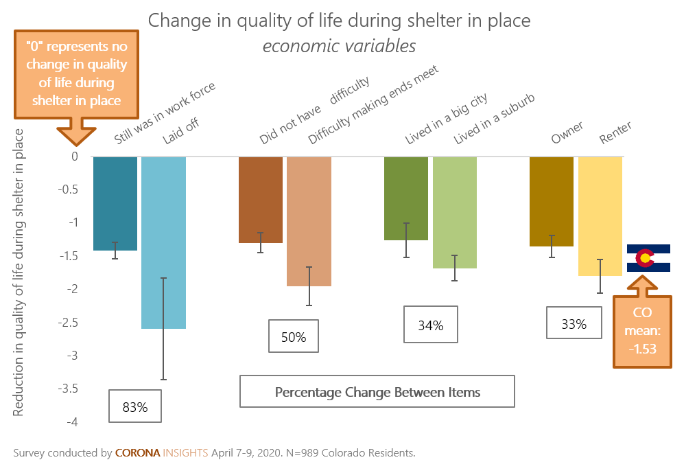
Perhaps unsurprisingly, our analysis shows that losing one’s job had the largest effect on quality of life change during the pandemic. Comparing a resident who was still in the work force to one who had been laid off resulted in an 83% reduction in quality of life during the pandemic. You will notice the whiskers attached to each estimate bar. These are 95% confidence intervals that provide an estimate of certainty that the population value lies within this range of the data. The confidence intervals on respondents who were laid off are larger because this group’s smaller sample size. Only 50 respondents from our survey sample reported losing their job. Twice as many reported a pay cut or being furloughed since March 1st, but these residents did not report a statistically different quality of life change than those still fully employed.
Respondents who said they had difficulty making ends meet as a result of COVID-19 also reported substantially larger decreases in their quality of life. Renters reported larger decreases than homeowners, and residents who said they lived in the suburbs had a harder time than those who said they lived in a large city. Next, we turn to the significant social and health variables from our model.
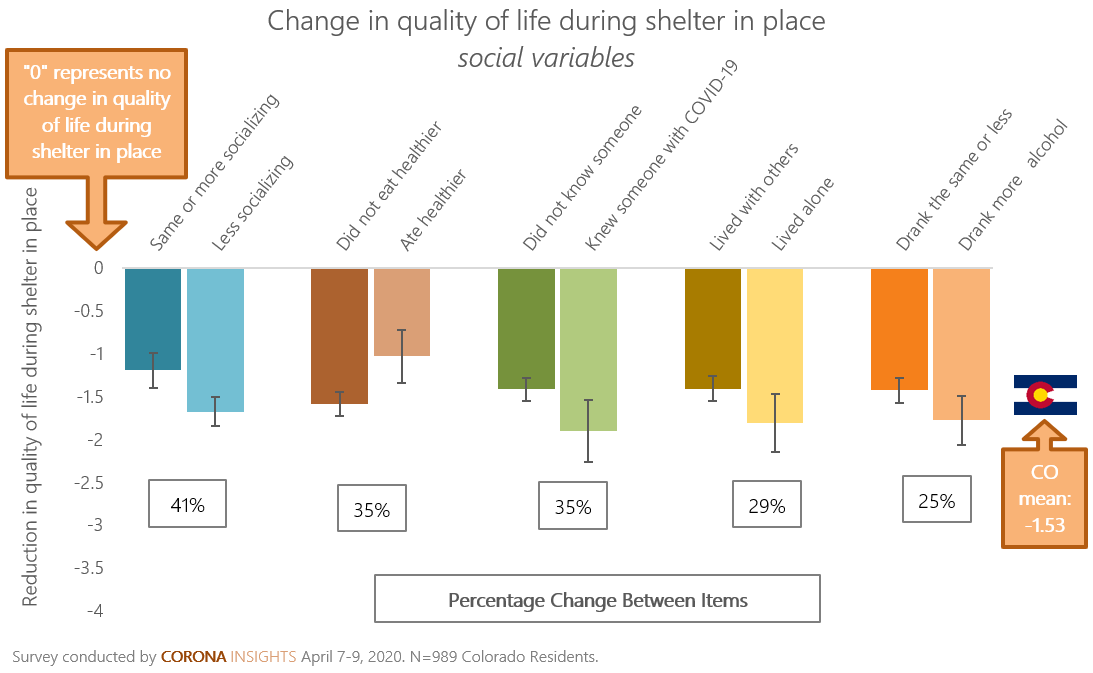
Amongst these variables, a reduction in time spent socializing appears to have the largest impact on quality of life during the pandemic. The fact that making more non-work video or phone calls had no effect on quality of life changes suggests these are imperfect replacements for in-person socialization. Similarly, Coloradans who lived alone reported larger decreases in wellbeing than those who lived with others.
While we did not ask if our respondents personally contracted COVID-19, those who were impacted by knowing someone with the virus had larger decreases in quality of life on average. In terms of behavioral health, exercising more during shelter in place was not associated with a statistical difference in wellbeing. However, those who said they were eating healthier at home fared better. Finally, respondents who admitted to drinking more alcohol during the pandemic reported steeper decreases in quality of life than those who drank similar amounts or less.
Overall, these data show that Colorado’s most vulnerable residents, those experiencing economic hardship and social isolation, have had the most difficulty during the pandemic. In these hard times we need each other more than ever. The Colorado COVID Relief Fund is providing aid to support the state’s communities and organizations disproportionately impacted by the outbreak. Please consider donating if you can.
How to Analyze the Data
In the next sections we provide a detailed write up for how we conducted this analysis and give guidance to anyone who wants to learn more about OLS regression.
There are many tools we could use to explain residents’ reported change in quality of life. Given that this outcome of interest, our dependent variable, has ordinal scores from -10 to 10, we would want to start by comparing the average change score across segments. Let’s say that we were particularly interested in understanding how renters were faring during COVID-19. The graph below presents the average change for Colorado’s homeowners compared to renters.
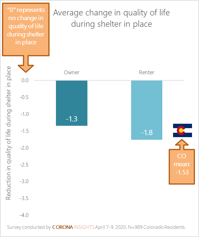
Looking at the means, we can see that it appears renters have been affected more than owners in that there has been a larger decrease in their average quality of life score, compared to homeowners. But what does this mean exactly? Is a difference of 0.5 large enough to say that this difference matters? We would want to run some statistical tests.
One of the most common tests in this realm would be a t-test. Like most statistical analysis tools, a t-test assesses the extent to which the difference we see here between these two groups is due to the independent variable (renter/owner status) or could be attributed to random chance. Running this test shows that this difference is in fact statistically significant. All that means here is that we can say there is less than a 5% chance that we would see a difference of this size, with these data, as a result of random noise. So, are we satisfied? Can we say that our research question about renters is answered? Maybe not. Renters and homeowners differ in a number of ways that might also impact their quality of life. For example, renters are younger, have lower incomes, and are more likely to live in urban areas. Our t-test results might be driven by any one of these variables. We cannot know without running more tests.
Regression models allow us to use multiple predictors, or independent variables, to explain our outcome of interest. Here we can control for important demographic and behavioral variables to place a line of best fit to our quality of life data. For example, we can observe the effect of renting compared to owning while controlling for a series of confounding traits. Even better, once we estimate our model, we can hold all other variables constant and assess estimated quality of life change across the range of any variable we are interested in. This is what we did to make the graphs in our key findings section. Regression allows us not only to see if different demographic and behavioral traits are associated with statistically significant changes in quality of life, but also lets us estimate and compare how large these changes are, all while ensuring relevant confounding factors are not biasing our conclusions.
Building a Regression Model
Now that we know our dependent variable is change in quality of life during COVID-19, we need to select a series of factors we think would drive different experiences for Coloradans. First and foremost, we want to control for key demographic traits. Variables like age, gender, household income, and race/ethnicity are foundational drivers of attitudes and behaviors. Including these in our model allows us to account for some of the ways these factors systematically shape what we say and do. As with most of our survey analysis, these data are weighted to represent the adult population of our intended sample universe, that of the state of Colorado.
Next, we want to include variables that we expect to influence quality of life in these unique times. We want to be selective in including these variables as throwing everything available into a regression model is bad practice and can cause statistical problems. Variables should only be included when we have good theory. This means prior research, usually qualitative or journalistic in nature, should drive our choices. As such, our background research pointed to a series of economic, social, and health factors. These include employment status, living situation, and changes to social/health behaviors. You can see the variables we decided to include below. In the next section we will discuss how to interpret all of this information.
| Table 2: Regression of Change in Quality of Life During Shelter in Place | ||
| B | SE | |
| A Large City (Omitted) | ||
| A Small City or Town | -0.101 | (0.193) |
| A Suburb Near a Large City | -0.426* | (0.163) |
| Outside of Any City or Town | -0.162 | (0.291) |
| Still in Work Force, No Pay Cut (Omitted) | ||
| Out of the Workforce as of March 1st | -0.241 | (0.182) |
| Took a Pay Cut or Was Furloughed | 0.148 | (0.235) |
| Laid Off | -1.175* | (0.398) |
| Essential Worker | 0.055 | (0.171) |
| Renter | -0.445* | (0.167) |
| Live Alone | -0.402* | (0.193) |
| Know Someone who has Been Diagnosed with COVID-19 | -0.486* | (0.195) |
| Has Difficulty Making Ends Meet as a Result of COVID-19 Situation | -0.653* | (0.174) |
| Is Doing Less Socializing during Shelter in Place | -0.483* | (0.138) |
| Making more Video and Phone Calls During Shelter in Place | -0.013 | (0.138) |
| Pursuing New/Existing Hobby | 0.146 | (0.162) |
| Ate Healthier During Shelter in Place | 0.555* | (0.171) |
| Drank More Alcohol During Shelter in Place | -0.352* | (0.167) |
| Exercised More During Shelter in Place | 0.038 | (0.143) |
| Spent More Time with Family During Shelter in Place | 0.140 | (0.142) |
| Read More During Shelter in Place | 0.166 | (0.141) |
| Pre-COVID-19 Quality of Life (Ordinal) | -0.454* | (0.042) |
| Age (Continuous) | 0.003 | (0.005) |
| Gender (Female) | -0.219 | (0.132) |
| Education (Ordinal) | 0.017 | (0.049) |
| Household Income (Ordinal) | -0.021 | (0.038) |
| White/Caucasian (Omitted) | ||
| Black/African American | 0.261 | (0.368) |
| Hispanic, Latinx, or Spanish Origin | -0.284 | (0.250) |
| Other Race/Ethnicity | -0.216 | (0.229) |
| Constant | 3.058* | (0.476) |
| Observations | 956 | |
| R2 | 0.27 | |
| Standard error in parentheses, * p < 0.05, survey weights based on 2018 ACS Colorado Adult Population, Variables are dichotomous unless otherwise noted. |
Interpreting Regression
The table above likely caused many readers to scroll at max velocity and could have even inspired some anxiety. Don’t panic! Each row of the table describes some critical information. Let’s start with the “Renter” row. Since renter is dichotomous (it has two values, owner=0 and renter=1), we can interpret its effect fairly simply. The coefficient, (represented in the B column) tells us how much moving one unit of the variable, in this case from being an owner to being a renter, changes the quality of life score on average. Since this coefficient is negative, we note that being a renter decreases the quality of life change score by -0.445. The * next to this number informs us that this change was statistically significant in the model. Note that this drop of 0.4 is quite close to the drop of 0.5 we saw from our t-test. All of that taken together provides more evidence to answer our renter research question. Even once holding all of these variables constant, renters reported a larger decrease in quality of life than homeowners.
In short, the B column tells how much, and in what direction (positive or negative number) a one unit increase in that row’s variable changes the quality of life score. The presence of a * tells us if that this change is statistically significant (not likely due to random chance). The SE column tells us the standard error used to calculate statistical significance.
Sometimes, we need to omit certain variables as a comparison category. For example, you will notice that A Large City doesn’t have a coefficient or standard error. This is necessary to estimate the effects of the next three variables. The model needs a reference category of which to compare the effect of living in a small city, suburb, our rural area. We can interpret the significant negative effect of living in A Suburb Near a Large City only to living in A Large City. This means that the quality of life of Coloradans who lived in suburban areas decreased significantly more than the quality of life of residents who lived in a large city. It does not allow us to say that the quality of life of Coloradans that lived in a suburb decreased significantly more than the quality of life of Coloradans that lived outside of any city or town.
This discussion only scratches the surface for what can be done with regression. Let us know if you have any questions about using this method in your future work!
The survey was fielded between April 7-9, 2020. Resulting data were cleaned and coded. Responses were weighted to represent the state of Colorado by geography and key demographic characteristics from the 2018 American Community Survey.
For further inquiry, please contact Corona Insights.